About me

• University of Nebraska, Omaha
  • B.S. Computer Science and Mathematics (2009)
  • M.S. Mathematics, Data Science (May, 2018)
• Software Engineer (2004-present)
• Flight Operations, U.S. Army National Guard (2000-2009)
  

  

  

  

A fun experiment

• Step 1: Pick a random percentage. e.g. 54%, 28%, 77%, etc.
• Step 2: Type that number into Google followed by “of Americans”
• Step 3: Follow rabbit hole for hours

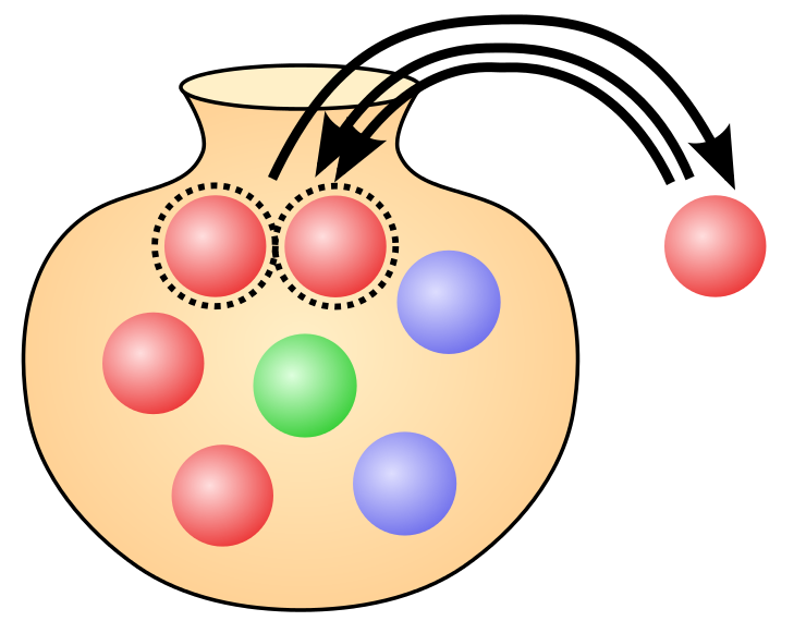
Simple random sample

• Pólya urn model
• With (SRSWR) or Without Replacement (SRSWOR)
  • With replacement - makes use of i.i.d. assumption
  • Without replacement - not i.i.d. but still exchangeable
• Requires access to the entire population

Sampling design

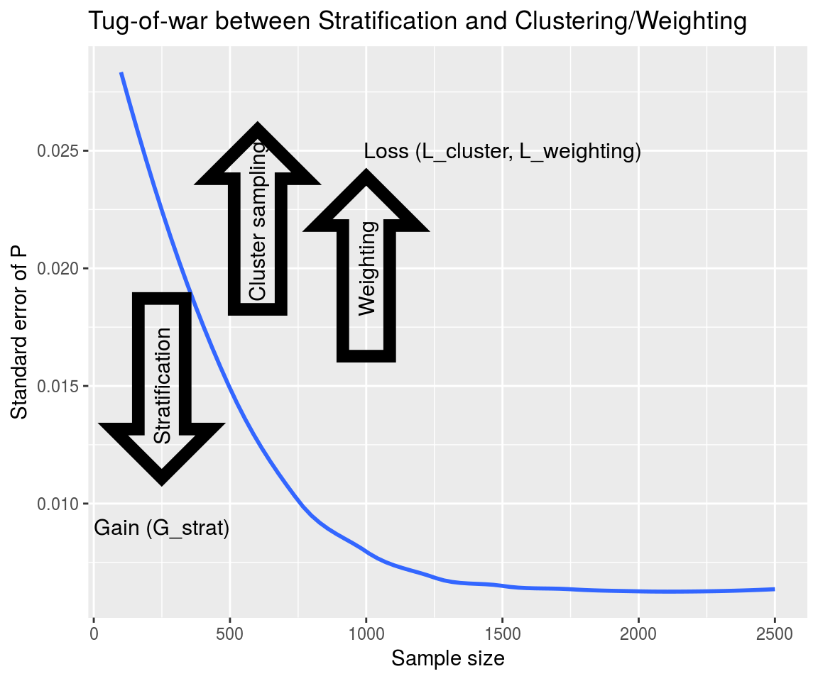
Design effects

Design effects

• “deft”
• Similar to variance inflation factor (VIF)
• Effective sample size

\[ D^2(\hat{\theta}) = \frac{SE(\hat{\theta})^2_{complex}}{SE(\hat{\theta})^2_{srs}} = \frac{var(\hat{\theta})_{complex}}{var(\hat{\theta})_{srs}} \]

\[ n_{eff} = \frac{n_{complex}}{d^2(\hat{\theta})} \]

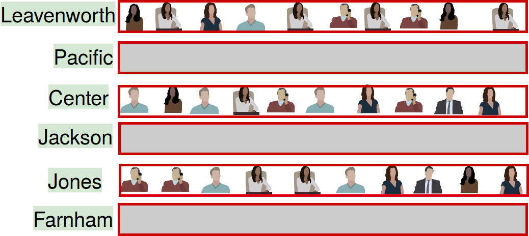
Clustering

• Grouping people by geographic regions
• SRS to choose a geographic region
  

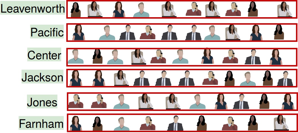
Clustering

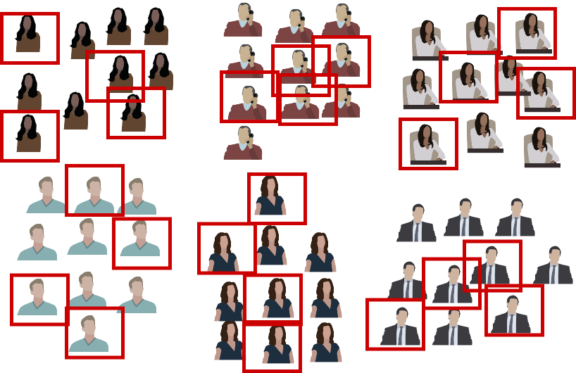
Stratification

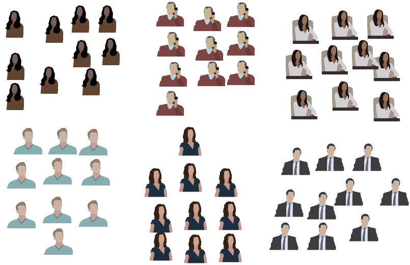
Stratification

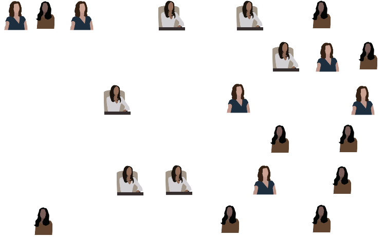
Weighting

• \(N = 51\)
  

Weighting

• \(N_{men} = 30\)
• \(p_{men} = \frac{30}{51} = 0.588\)
  

Weighting

• \(N_{women} = 21\)
• \(p_{women} = \frac{21}{51} = 0.412\)
  

Weighting

• \(N_{women} = 21\)
• Women Odds Ratio: \(\frac{p_{women}}{p_{men}} = \frac{0.588}{0.412} = 1.427\)
• Men Odds Ratio: \(\frac{p_{men}}{p_{women}} = \frac{0.412}{0.588} = 0.701\)

H-CUP Nationwide Inpatient Sample

• Healthcare Cost and Utilization Project
• Must be purchased

NIS Sampling Design

• 1988-2011: 100% sample of 20% of HCUP hospitals
• 2012-present: 20% sample of 100% of HCUP hospitals

NIS Complex Survey Design

• Clustered on hospital ID
• Weights included in discwt field for national estimates
• 1988-2011: Stratified by census region and bed size
• 2012-present: Stratified by census division and bedside
  • Region 1 (Northeast)
    • Division 1 (New England) -Division 2 (Mid Atlantic)
  • Region 2 (Midwest)
    • Division 3 (East North Central)
    • Division 4 (West North Central) (incl. Nebraska)
  • Region 3 (South)
    • Division 5 (South Atlantic)
    • Division 6 (East South Central)
    • Division 7 (West South Central)
  • Region 4 (West)
    • Division 8 (Mountain)
    • Division 9 (Pacific)

NIS dimensions

• Big data?
• Definitely large data
• ~3GB per year (raw CSV)

Importance of survey design

• Treating as SRS

summary(lm(los~age, data=cdiff))

## 
## Call:
## lm(formula = los ~ age, data = cdiff)
## 
## Residuals:
##    Min     1Q Median     3Q    Max 
## -14.19  -7.12  -3.98   2.27 349.01 
## 
## Coefficients:
##              Estimate Std. Error t value Pr(>|t|)    
## (Intercept) 14.190744   0.187955   75.50   <2e-16 ***
## age         -0.043275   0.002687  -16.11   <2e-16 ***
## ---
## Signif. codes:  0 '***' 0.001 '**' 0.01 '*' 0.05 '.' 0.1 ' ' 1
## 
## Residual standard error: 13.94 on 73264 degrees of freedom
## Multiple R-squared:  0.003528,   Adjusted R-squared:  0.003514 
## F-statistic: 259.4 on 1 and 73264 DF,  p-value: < 2.2e-16

Importance of survey design

• Accounting for survey design with R survey package

library('survey')

cdiff.design <- svydesign(ids = ~hospid, data = cdiff, weights = ~discwt,  strata = ~nis_stratum, nest=TRUE)
summary(svyglm(los~age, design=cdiff.design))

## 
## Call:
## svyglm(formula = los ~ age, design = cdiff.design)
## 
## Survey design:
## svydesign(ids = ~hospid, data = cdiff, weights = ~discwt, strata = ~nis_stratum, 
##     nest = TRUE)
## 
## Coefficients:
##             Estimate Std. Error t value Pr(>|t|)    
## (Intercept) 13.95231    0.55033  25.353  < 2e-16 ***
## age         -0.04657    0.00637  -7.311 6.27e-13 ***
## ---
## Signif. codes:  0 '***' 0.001 '**' 0.01 '*' 0.05 '.' 0.1 ' ' 1
## 
## (Dispersion parameter for gaussian family taken to be 180.579)
## 
## Number of Fisher Scoring iterations: 2

SRS vs. complex design

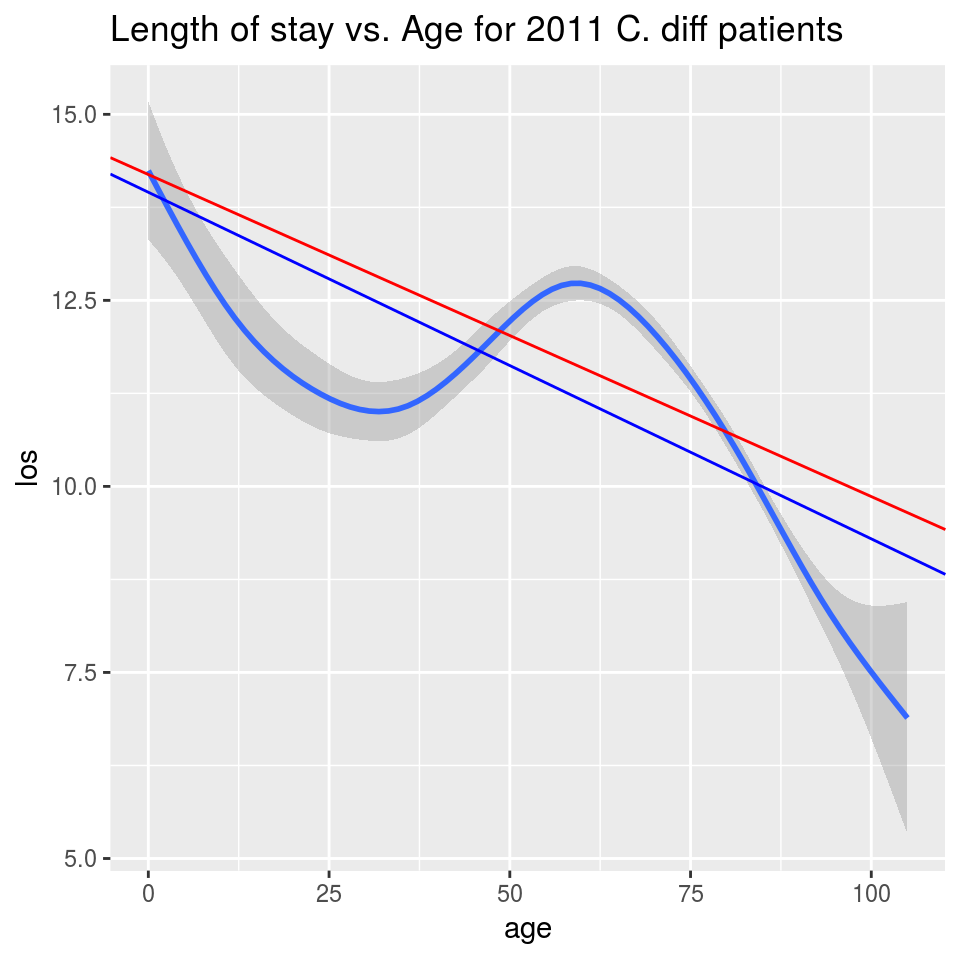
SRS line in red, complex design in blue

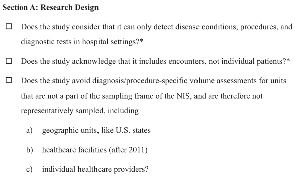
Research design checklist

• Khera and Krumholz, 2017

  

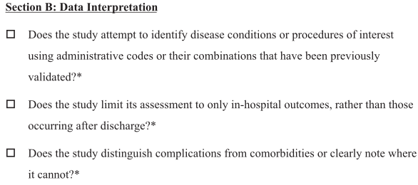
Data interpretation checklist

• Khera and Krumholz, 2017

  

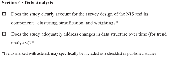
Data analysis checklist

• Khera and Krumholz, 2017

  

Sources and Further Reading

• Heeringa, S., West, B. T., Berglund, P. A., Applied Survey Data Analysis, 2nd Ed., CRC Press (2017)
• Kalton, G., Introduction to Survey Sampling, SAGE Publications (1983)
• Khera R. and Krumholz H., With Great Power Comes Great Responsibility: Big Data Research From the National Inpatient Sample, Circulation: Cardiovascular Quality and Outcomes (2017)
• Lumley, T. R Package ‘survey’, (2018)